Namaste! In my last blog-post I wrote about Deep Learning and diseases. I showed a way to use a simulator in order to generate a large data-set for a Neural Network that analyzes diseases. Because you need large data-sets for Deep Learning, right? This is a good moment to focus on Machine Learning and Deep Learning.
The statement about large data-sets is only half of the truth. Generally Deep Learning is understood as training deep Neural Networks. „Neural Networks that have a lot of hidden layers.“ Using Deep Learning technologies like Keras and TensorFlow for shallow Neural Networks is still considered Deep Learning. In my world.
The truth about Machine Learning and Deep Learning under consideration.
It is true that Deep Learning only gets to full speed properly when you have a large dataset. That is where the whole success comes from. Nowadays there is a lot of data available. And everyone knows: „Use traditional Machine Learning, when you do not have that much data.“ I personally do not really share that opinion.
In this article I will compare two generations of Machine Learning algorithms. The first is k-Nearest-Neighbor implemented with scikit-learn. The second is Deep Learning with Keras. We will do this to explore the old notion, that all roads lead to Rome.
As always, you will find the full source-code in my GitHub repository. Feel free to toy with the code. And send my your comments if you like. Looking forward!
First things first. Let us set up our Python project.
Again and as always in my tutorials series, let us start right away and import everything that is necessary:
import numpy as np
import matplotlib.pyplot as plt
import pandas as pd

from sklearn.model_selection import train_test_split
from sklearn.datasets import load_iris
from sklearn.neighbors import KNeighborsClassifier

import keras
from keras import models
from keras import layers
from keras.utils import to_categorical
Who are our favorite actors on stage? NumPy is THE package for Python scientific computing. Matplotlib is THE package for 2D plotting. pandas is THE Python data analysis library. scikit-learn is THE Python Machine Learning library. And of course Keras is THE Deep Learning library.
As a Machine Learning and/or Deep Learning enthusiast you might know most if not all of them. As a newbie know that all of them would be worth having a deep look at.
The main()-method.
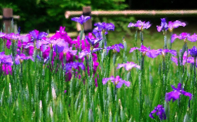
It is time for me to tell you what is going to happen next. I kept you in the dark for a while. Kinda intentionally. We are going to create a classifier for flowers. Both in scikit-learn and in Keras. The Iris Flower Data-Set dates back to 1936. It contains 150 samples of three subspecies of Iris, the national flower of Croatia.
The data-set is a good example for a multi-variate collection of data. It basically maps four variables to three classes of flowers. In our tiny little testbed-application, we will do three things. Analyzing the data, applying a traditional Machine Learning algorithm, and applying Deep learning. This is the main()-function:
def main():

    # Analyze the data-set.
    analyze()

    # Apply Machine Learning.
    machine_learning()

    # Apply Deep Learning.
    deep_learning()
As usual, before anything else, it is Data Science time! Analyze first, train after that!
Let us dissect our data-set. Well, at least a little… Minimally invasively.
It is always advised to do a data analysis before starting any Machine or Deep Learning endeavor. Why? Very simple. It is good to know what you are dealing with. How is it structured? What kind of information is encoded? How clean is it? Is it well balanced? Let’s find out:
def analyze():

    print("Analyzing data-set...")

    iris_dataset = load_iris()
    x_train, x_test, y_train, y_test = train_test_split(iris_dataset["data"], iris_dataset["target"], random_state=0)

    print("x_train shape:", x_train.shape)
    print("y_train shape:", y_train.shape)
    print("x_test shape:", x_test.shape)
    print("y_test shape:", y_test.shape)

    iris_dataframe = pd.DataFrame(
        x_train,
        columns=iris_dataset.feature_names
    )
    pd.plotting.scatter_matrix(
        iris_dataframe, c=y_train,
        figsize=(15,15), marker="o",
        hist_kwds={"bins": 20}, s=60, alpha=0.8)
    plt.show()

    print("")
You will see two things. Some console-output. And a plot. This is what the console has to say:
Analyzing data-set...
x_train shape: (112, 4)
y_train shape: (112,)
x_test shape: (38, 4)
y_test shape: (38,)
It basically says, that our dataset is comparatively small. We knew this from the beginning. A data-set with 150 samples is basically nothing. So we won’t train it on a GPU. Promised. Fortunately we only want to classify flowers and not create an extensive object recognition system. In this domain we will get good results without Big Data. Promised.
The plot is a so called scatter matrix. This matrix uses all features (variables) of a dataset and consideres them in pairs. Each pair is then plotted as a 2D image showing the distribution of their values. This gives you a good hint about how separate the classes are. This gives you a good grip on the decision, which Machine Learning algorithm to use. See for yourself:

Obviously, the values are clearly seperatible. Thank Krishna. This is a good start for our classifiers!
Tradition is not the worship of ashes, but the preservation of fire.
Yes, that was some random quote by Gustav Mahler. You know, Machine Learning and Deep Learning are not two different pairs of shoes. Deep Learning is only one special Machine Learning Algorithm. One amongst many, many other. This means that Deep Learning is Machine Learning. But not all Machine Learning is Deep Learning. Logics at its best.
When I refer to traditional Machine Learning, I mean all those algorithms that have nothing to do with Deep Learning. For example Random Forests, Support Vector Machines and of course k-Nearest-Neighbors. The latter is one of the most simplest Machine Learning algorithms. And yet it is very effective. It classifies a sample with respect to its nearest neighbors. Distance. Simple as that!
Here is the code. Straightforward and elegant:
def machine_learning():

    print("Applying k-Neighbors algorithm...")

    # Loading the data-set.
    iris_dataset = load_iris()

    # Train-test-split.
    x_train, x_test, y_train, y_test = train_test_split(iris_dataset["data"], iris_dataset["target"], random_state=0)

    # Initializing the classifier.
    knn = KNeighborsClassifier(n_neighbors=1)

    # Training the classifier.
    knn.fit(x_train, y_train)

    # Evaluating the model.
    test_accuracy = knn.score(x_test, y_test)
    print("k-Neighbors test-accuracy:", test_accuracy)
    print("")
What we see here is quite trivial. Firstly, the Iris-data-set is loaded. Then we do the train-test-split. Remember that this is standard practice in Machine Learning. We train our model on the training set and we evaluate its capability to generalize on the testing set. Think about overfitting. This is how we measure it.
After the split, the k-Nearest-Neighbor classifier is instantiated. In our case k is 1, which means that the closest neighbor wins. I cannot get simpler. Then the model is being fit. In this approach is not really more than storing the training-data. There is no magic training involved.
And finally, we evaluate the model against our test-set. This is the output:
Applying k-Neighbors algorithm...
k-Neighbors test-accuracy: 0.9736842105263158
Out classifier works with a test-accuracy of 97%! This is really good! And please, count the lines of code. Now, let us solve the same problem again. But this time with Deep Learning. Like an axe in the woods, how we Germans say.
Tradition becomes our security, and when the mind is secure it is in decay.
Yea, this was a quote by Krishnamurti. We will now consider „modern“ Machine Learning. Mind the quotes around the word modern. Neural Networks are an old hat. But they proved to be very effective only quite recently. Enter Keras – the Lego building blocks toolbox when it comes to Deep Learning. Here is the code:
def deep_learning():

    print("Applying Deep Learning...")

    # Loading the data-set.
    iris_dataset = load_iris()
    input_data = iris_dataset["data"]
    output_data = iris_dataset["target"]

    # Applying a to_categorical encoding.
    output_data = to_categorical(output_data)

    # Train-test-split.
    x_train, x_test, y_train, y_test = train_test_split(input_data, output_data, random_state=0)

    # Normalizing the data.
    minimum = np.min(x_train)
    maximum = np.max(x_train)
    x_train = (x_train - minimum) / (maximum - minimum)
    x_test = (x_test - minimum) / (maximum - minimum)


    # Creating the model.
    model = models.Sequential()
    model.add(layers.Dense(40, input_shape=(4,)))
    model.add(layers.Dense(3, activation="softmax"))

    # Compiling the model.
    model.compile(
        loss="mse",
        optimizer="rmsprop",
        metrics=["accuracy"]
    )

    # Training the model.
    model.fit(x_train, y_train, epochs=100, batch_size=8, verbose=0)

    # Evaluating the model.
    _, test_accuracy = model.evaluate(x_test, y_test)
    print("Deep Learning test-accuracy:", test_accuracy)
    print("")
Well, loading the data is almost god-given. After that we have to do some magic. We do a categorical encoding of the labels. A label 3 in a three-classes-scenario becomes the vector 0 0 1 – this makes it easier for Neural Networks. This is a standard practice.
The train-test-split is the same. There are no differences here. 75% train, 25% test.
Neural Networks work well with floating point input values that are quite small. Going for values between 0.0 and 1.0 is always a good choice. That is why we normalize both the train and test input values with numbers that we derived from train. Keep in mind not to leak any information about test into train. That is why we compute the minimum and the maximum only from train, and normalize both train and test using those numbers.
Now comes the good part – modelling, training, evaluating. We will use a two-layer fully-connected Neural Network. The hidden layer width is 40. Determined empirically. The input-size is four, which is the number of features. And the output-size is three, which is the number of classes. We will use Mean Squared Error as the loss function and we will use RMSprop as optimizer.
Training is straightforward. We fit the net in 100 epochs with batch-size 8. What would the test-accuracy be after a couple of seconds of training? See for yourself:
Applying Deep Learning...
38/38 [==============================] - 0s 226us/step
Deep Learning test-accuracy: 0.9736842073892292
The test-accuracy is about 97%, which is the same as in the k-Nearest-Neighbor approach. Very good! And even without Big Data!
What have we learned about Machine Learning and Deep Learning?
I admit, this was not a showdown between traditional Machine Learning and Deep Learning. I never intended this. Both are equally valuable. In our world there is no space for a thing such as a showdown. The point I wanted to make is that Deep Learning can be applied to very small data-sets. You just would not create very huge Neural Networks to train on the data. You would go for smaller, shallow ones. I guess, I proved that point. Thanks for reading!
Stay in touch.
I hope you liked the article. Why not stay in touch? You will find me at LinkedIn, XING and Facebook. Please add me if you like and feel free to like, comment and share my humble contributions to the world of AI. Thank you!
If you want to become a part of my mission of spreading Artificial Intelligence globally, feel free to become one of my Patrons. Become a Patron!
A quick about me. I am a computer scientist with a love for art, music and yoga. I am a Artificial Intelligence expert with a focus on Deep Learning. As a freelancer I offer training, mentoring and prototyping. If you are interested in working with me, let me know. My email-address is tristan@ai-guru.de - I am looking forward to talking to you!